How to connect real-time optimization to a predictive multivariable controller
Today's applications present a number of problems with connecting a real-time optimization (RTO) to a predictive multivariable controller (PMC). The first arises from the inherent model mismatch between the nonlinear, first-principle, steady-state models employed by the RTO and the empirical, linear dynamic models used by the controller. At best, the controller model is identified in the region where the RTO typically operates. In this region, the steady-state gains of the controller should be similar to those in the nonlinear model of the RTO. Unfortunately, comparing these gains is not possible without special effort because the independent variables in these two models are not the same, which implies the controlled variables (CVs) are not in the right context. The independent variables in the controller are the manipulated variables of the controller. The independent variables in the RTO are determined by the kinetic, thermodynamic and equilibrium relationships, which are embedded in the correlations that are chosen for the models.
Charles Cutler is president, Don Golden is technical support consultant, and Charles Johnston is APC Consultant at Cutler Technology. They may be reached at (832) 451-4452 or [email protected].
The controller updates its parameters to match the plant measurements on a minute-to-minute basis. On the other hand, the RTO waits until the process reaches steady state before it performs a parameter update. A complex process usually takes a number of hours to reach steady state, so the parameter update for the RTO is at least two orders of magnitude less frequent than the controller. The PMC gets around the steady-state problem by using its prediction to estimate the steady-state conditions upon which it bases its optimization. As a result, the optimization based in the PMC will at best only approximate the RTO.
Figure 2: Changing the high limit on DPDEPROPPV, the differential pressure (DP) across the column, from 3.62 to 3.55, moves the controller into an infeasible operating region (Figure 6b).
The usual procedure for implementing an RTO is to provide external targets (ETs) to the controller. Most multivariable controllers' optimizers are based on the linear programming (LP) algorithm that sets the goals for the controller's calculations. Imposing the ETs forces the controller's LP optimizer to move the entire model mismatch into the remaining degrees of freedom that are not driven by an ET. A basic requirement of a linear program is the number of active constraints must be equal to the number of manipulated (independent) variables in the controller. If 60% of the degrees of freedom for the controller are used up on ETs, then the controller's LP will solve its economic problem based on the remaining 40% where the entire mismatch has been concentrated. The inherent problems with the mismatch can cause the controller's LP to be infeasible, which usually forces the number of ETs to be reduced to 20-40% of the degrees of freedom.
Eliminate the Competition
Rather than have the controller trying to resolve the model mismatch by moving the process around, a better solution would be to have the controller focused on satisfying the ETs from the RTO, and only move the process for this purpose. In effect, the controller should become subservient to the RTO optimizer and not compete with the RTO solution.
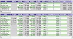
Figure 3: Case 3 sets a scenario showing the differences between ranking and smearing (distributing the infeasibilities with minimum movement) to handle the infeasibilities in the controller's linear programming.
As the number of ETs increases, the controller will have a more difficult time finding a feasible solution from its LP. The general approach to deal with this issue is to rank the control variables in order of importance, and drop out the lower-rank variables as they become active constraints. This approach will eventually allow the LP to become feasible. The problem with this method is that the control variable constraints are based on meeting product specifications, equipment limitations and safety considerations. Dropping a constraint causes the LP to completely disregard the variable.
Figure 4: For Case 4, the upper limit on DPDEPROPPV was changed from 3.62 to 3.55, which caused the controller's LP to be infeasible. The controller distributed the infeasibilities based on the RIs. Removing the lowest ranked controlled variable, DC3FEEDPV, didn't remove infeasibility because the lower limit on DC3FEEDSP became active at 21.2 MBPD.
Dropping out a constraint also will cause the LP to find a new solution that may not be close to its previous one. Such perturbations cause the controller to appear unstable. A better solution is to keep all the constraints and allow their violation to be based on their relative importance (RI). Constraint violations are dealt with in an elastic manner as defined by the RIs of the violated constraints. This approach gives the controller greater information, which allows it to grade the amount of the violation for a particular constraint relative to the remaining constraints, rather than treating the constraint as an on/off switch.
We've developed a PMC that addresses these issues in an innovative way by smearing [distributing the infeasibilities] with minimum movement." In the simplest terms, the controller drives the process to the external targets, while minimizing extraneous movement of the process. The controller uses its degrees of freedom to reject disturbances and respond to changes in ETs, but it is not using its own optimizer in conflict with the RTO optimizer. Thus, the controller minimizes the movement of the independent variables to keep the controller solution within its constraints and at its external targets, or as close as possible in the context of their specified relative importance, whether the solution is feasible or not. In effect, the RTO specifies through the external targets where the operation is the most economic, while the controller minimizes the movement of the manipulated variables to get the process as close as possible to the RTO objectives. This scenario moves the process gently in and out of the feasible operating region without the disruption caused by dropping out control variable constraints. It avoids the poor performance of the controller caused by its objective function having different gains from those in the RTO's objective function. The conflict between the two optimizers is eliminated by using only the RTO's economic solution.
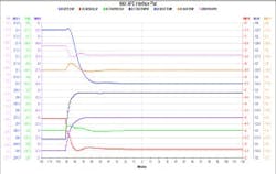
Figure 5: In Case 5, a feasible solution is achieved by dropping constraints, but movingDC3FEEDSP to its upper limit, which was 2.5 MBPD above the CV limit set by the optimizer, and DC3BOTTEMP is 4.0600 DEGF below its controlled variable limit (Figure 6a).
Proof on Depropanizer
A simulation of a depropanizer column illustrates these points. The pressure control on the column is done by bypassing part of the overhead vapor around the condensers and into the overhead accumulator. The temperature control of Tray 5 is accomplished by adjusting the reflux to the column. The reboiler heat is supplied by the flow of an external liquid stream. The feed rate to the column is on flow control. The PVs of the manipulated variables are specified as dependent control variables to illustrate how they respond to the setpoint changes, and to permit RIs to be placed on the variables to permit them to be infeasible. Manipulated variables are not allowed to exceed their limits under any circumstance.
Figure 6a: A feasible solution is achieved by dropping constraints, but DC3FEEDSP moved to its upper limit, which was 2.5 MBPD above the CV limit set by the optimizer, and DC3BOTTEMP is 4.0600 DEGF below its controlled variable limit.
Figure 6a: A feasible solution is achieved by dropping constraints, but DC3FEEDSP moved to its upper limit, which was 2.5 MBPD above the CV limit set by the optimizer, and DC3BOTTEMP is 4.0600 DEGF below its controlled variable limit.
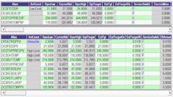
Case 1 illustrates the controller with four external targets after the controller has reached steady state (Figure 1). The controller is feasible with all four of its degrees of freedom set with the four external targets. The external target, current value and steady-state target have the same value for each of the four external targets. The relative importance (RI) of each controlled variable at steady state is displayed, and the differential pressure across the column (DPDEPROP) has transition zones that range from being totally unimportant at a low value to being very important as it approaches the upper limit.Case 2 (Figures 2 and 6b) illustrates the effect of moving the controller into an infeasible operating region by changing the high limit on the differential pressure (DP) across the column (DPDEPROPPV) from 3.62 to 3.55. The RI for the DP at the upper limit and above moved to 0.01. In effect, 0.01 psi on the DP was as important as 3.0 MBPD of feed, 0.70 DEGF on the over head temperature, 2.0 DEGF on the bottom temperature, and 0.2 PSI on the top pressure. The controller did not give up on the DP high limit. On the ETs, it changed -0.2893 MBPD on the feed, 0.0675 DEGF on the top temperature, -0.1929 DEGF on the bottom temperature and 0.0193 PSI on the top pressure. The controller's LP distributed the infeasibility based on the constrained CV's RIs.
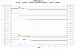
Figure 6b shows the response of the key variables when the controller became infeasible. DPDEPROPPV moved down gracefully to its new upper limit. The three curves at the top of the graph are the dependent controlled variables and the four curves at the bottom of the graph are the independent manipulated variables. The graph shows 60 minutes of past history and 60 minutes of the projected future response. Also, the vertical line in the center of the graph shows the current time.
Case 3 (Figure 3) sets a scenario showing the differences between ranking and "smearing with minimum movement" to handle the infeasibilities in the controller's LP. The LP is based on the predicted steady state for the controller and effectively provides the multivariable controller with its set points. The upper and lower limits on the ET variables are set to the value of the ET variables in Case 1. The formulation of Case 3 without ETs gives the same results as Case 1 with ETs when the controller's LP is feasible.
In Case 4 (Figure 4), the normal control mode was in effect using its regular costing and without the controller minimizing movement of the manipulated variables. The case had no ETs. The upper limit on DPDEPROPPV was changed from 3.62 to 3.55, which caused the controller's LP to be infeasible. The controller distributed the infeasibilities based on the RIs. Here, the ranking of the controlled variables was emulated by removing DC3FEEDPV with the service switch. Turning off the switch effectively took the lowest ranked CV constraint out of the controller that was at a constraint. The infeasibility for the problem was not removed because the lower limit on DC3FEEDSP became active at 21.2 MBPD.
Figure 6b: The differential pressure across the column (DPDEPROPPV) moved down gracefully to its new upper limit.
Case 5 (Figures 5 and 6a) illustrates that taking DC3BOTTEMP out of service allows the LP to find a feasible solution. DC3BOTTEMP was an active CV constraint—the second CV from the bottom in the ranking list. Here, the order of the ranking list is the same as the RI list. With both DC3BOTTEMP and DC3FEEDPV out of the controller, the feasible LP solution moved the DC3FEEDSP to its upper limit, which was 2.5 MBPD above the CV limit set by the RTO, and also moved DC3BOTTEMP by 4.0600 DEGF below its CV limit. The other two constraints set by the RTO were back at their targets as the LP solution became feasible.In contrast, the "smearing with minimum movement" of the projected steady state only (Case 2) moved the feed -0.2893 MBPD, -0.1929 DEGF on the bottom temperature, 0.0193 PSI on the top pressure and 0.0675 DEGF on the top temperature. A direct comparison of the two methods of handling infeasibilities is shown in Figures 6a and 6b. Figure 6a shows the instability that ranking can create by dropping active constraints completely out of the LP. Figure 6b, with "smearing and minimum movement," is shown on the same scale.
Summary
In the demonstrated solution, when the controller is receiving targets from an optimizer, it goes into a minimum movement mode for the manipulated variables, and the objective function for the optimizer continues to use the RIs associated with the dependent variables. This permits the distribution of the infeasibilities across all the active constraints based on their relative importance. From a control point of view, this is more stable, since it relaxes all the active constraints by just enough to get within the constraints, while minimizing the movement to the MVs steady state objectives.
Figure 1: In Case 1, the external target, current value and steady-state target have the same value for each of the four external targets. The relative importance (RI) of each controlled variable at steady state is displayed, and the differential pressure across the column (DPDEPROP) has transition zones that range from being totally unimportant at a low value to being very important as it approaches the upper limit.

Leaders relevant to this article:

