Greg: We conclude our discussion of distillation control best practices with Mark Darby of CMiD Solutions and Doug Nicholson of Spiro Control by offering additional knowledge to provide essential guidance on how to make the most out of simulation and optimization opportunities.
Simulations of distillation columns can offer incredible benefits in finding, implementing, improving and optimizing the best control system, but the effort to achieve the high-fidelity dynamic simulation needed is considerable. The use of simulation software with advanced modeling objects for a wide spectrum of equipment designs is especially important. The user can then concentrate on getting and entering the physical parameters of equipment (e.g., volumes, diameters, number and geometry of trays) and the physical properties, flows and operating conditions of all streams and fluids in the equipment.
The time to steady state can be hours or days. Consequently, dynamic simulations require patience and some fixed speedup to see the final responses of the control system. Variable speed up seen in some simulations is not a viable option unless all the control system dynamics have the same speed up. This is rarely possible because often the dead times and time constants associated with the control system are proportionally reduced and the control tuning changed accordingly (e.g., PID gain and rate time decreased and PID reset time increased). This is problematic in most cases.
There has also been a propensity for the need to completely start over in creating a dynamic model and the dynamic model falling short in terms of the intensity of detail in the process and equipment models seen in steady-state models. For this and many other reasons, steady-state simulations are preferably used as a starting point to find the best temperature sensor locations (e.g., best tray) and the process gains that are essential for PID feedback and feedforward gains, as well as relative gain analysis (RGA) to determine the best pairing of controlled and manipulated variables and decoupling needed. The matrix relative gains and condition number are also used for model predictive control design.
Steady-state simulations can continue to be used for optimization. Dynamic simulations can be checked to be consistent with steady state simulation and the task of the dynamic simulation focused on completing the parameterization of the PID and model predictive control systems and providing a simulation for testing, training, diagnostics and innovations, including procedure automation (e.g., state-based control) to deal with startup and abnormal operation.
Mark and Doug, what are some of the other important aspects in the development and use of simulations?
Mark: A steady-state simulation can also help evaluate various control strategies. Say your concern is unmeasured disturbances in the feed composition. You can, for example, determine open-loop gains holding different manipulated variables constant such as reflux, boil-up, distillate or a tray temperature. These simply become different specifications for the simulation. Candidate schemes are those with the smallest disturbance gains.
Doug: I like to use steady-state simulation to check composition gains to independent variables (manipulated and disturbance), especially when there is uncertainty in the identified gains due, for example, to a long response time. It is important to specify the simulation with the same degrees of freedom (manipulated and disturbance variables) as the actual column. To get around possible inaccuracies in calculating the gain (slope), with either too small or too large a change, I like to make multiple simulation runs varying each independent variable over a selected range while keeping others constant. Then, from a plot or equation fit of the composition to the independent variable, determine the gain. From the plot, I can also determine how much the gain varies. If significant, a characterizer can be fit to the simulation data. This approach is known as a linearizing transformation in the MPC community.
Other examples of where a steady-state simulation can be useful include determining the gain for a pressure compensated temperature by varying column pressure at constant composition or getting the factor for an internal liquid calculation. For example, simulation can be used to develop a soft sensor model in determining the inputs and/or fitting the model.
Greg: Soft sensors can provide composition measurements based on steady-state simulations without the dynamics from the process and the analyzer. The soft sensors can be corrected by a bias that is a fraction of the difference between the prediction by the soft sensor with inclusion of dynamics and a validated analyzer result. The dynamic compensation of the soft sensor is helped by the identification of the dynamics via a dynamic simulation in a digital twin that has the sample transportation delay, cycle time, analysis time, and multiplex time. The dynamic simulation in a digital twin can be extended to include MPC whose targets are the actual controller outputs, controlled variables are the digital twin controller outputs, and manipulated variables are key dynamic simulation parameters. The extensive nonintrusive development, tuning, and testing of soft sensors and controls possible with simulations in digital twins and particularly the automated adaptation of dynamic simulations is not commonly recognized.
Mark: Setting up a dynamic simulation requires more effort than a steady-state simulation and includes specification of vessel sizes, valves and the regulatory PID controllers. Because it is dynamic, it takes time to integrate the equations and for the response to evolve. The simulation time also depends on whether and how much the simulation can be sped up. A dynamic simulation, particularly if one is already available, can be used to evaluate a design or change in the regulatory control strategy, thereby avoiding the associated challenges of doing so on the live plant or before the plant is built. It can be a useful check for a design based solely on steady-state analysis. Dynamic simulation can also be used to introduce and train operators on MPC or to get initial dynamic models for MPC or tuning of PID controllers.
Greg: A digital twin where the actual control system configuration and operator interface is used with a dynamic simulation eliminates the huge task and unavoidable errors associated with an emulation, where the control system and interface is programmed to try and duplicate what is in the plant. The ability to import and download the actual control system modules and utilize the actual operator graphics and data historian in the control room translates to much better testing, tuning, training and maintenance resulting in much greater, consistent and reliable operator and control system performance.
As a final topic, let’s discuss the optimization of distillation columns.
Mark: It can be appropriate to consider optimization if there are trade-offs that change over time that cannot be achieved with a constraint-pushing strategy such as with MPC. These include variations in economics or operation, which often occurs when reactors are used upstream of distillation columns. The optimization may be performed online or offline. When online, targets are normally downloaded automatically (closed loop) to the control system, often to a MPC to ensure constraints are enforced between optimization executions. With open loop, the optimization targets are implemented manually, usually by the operator. Benefits are naturally greater when the optimization is performed automatically in closed loop with model updates to match current plant operation.
Doug: A range of model approaches have been used since computers were first deployed in operating plants. Early on simplified models were the only possibility due to computer limitations – in terms of both processing speeds and memory. Models of increased rigor and complexity have been increasingly used as these limitations were removed and large-scale solvers came on the scene. Over the past 25 years, online optimization has been mostly implemented with rigorous steady-state models based on first principles, including mass and energy balances, physical properties, and vapor-liquid equilibrium.
Greg: I know the necessary support requirements for these optimizers has been difficult for many companies. Are there other challenges, and what are new trends?
Doug: True. The specialized nature of the required skill set has proven difficult for many companies to foster and maintain. The other challenge is the wait time required for the process to become to update the steady-state model and rerun the optimization. This limits how often the optimizer can be executed.
Today we are seeing the level of modeling rigor more focused on the required model accuracy and sensitivity of the optimum. More recently, dynamics have been incorporated into the model update step. The optimization is still steady-state, but because the model update accounts for dynamics, it removes the necessity of the steady-state wait time, thereby allowing the optimization to be scheduled on a fixed and faster time internal. Simpler models have been used with this approach, owing to faster model updates. This has enabled larger optimization envelopes and a tie-in to operational planning, where feeds and inventories can be coordinated.
Mark: There are other benefits and applications of an online model such as performance monitoring of key performance indicators leading to earlier detection of process problems or performing what-if scenarios. This might be better termed an operational twin. In this area, we are seeing the use of hybrid models that include both data driven and first principles components. As with online optimization, higher benefits will accrue when the model is updated in real time to reflect changing process conditions.
Greg: For much more on how simulation is used and its importance, see the Control article “Simulation enhances career and system performance,” the Control Talk Column “Simulation breeds innovation” and ISA Mentor Program Q&A post “How is simulation leverage for Qualification and Management of Change.”
Top 10 reasons to not do simulations
10. You like spending nights and weekends in the plant.
9. You don’t want challenges to your solutions.
8. You only want to work with real stuff.
7. Simulation results that disagree with your thinking are “fake news.”
6. Simulation people are so “off the grid” you have no idea what they are talking about.
5. You just want to do “your thing.”
4. Artificial intelligence is your backup.
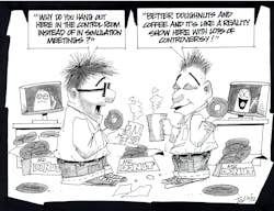
3. You would rather the project fund more food and doughnuts and more of your time and travel.
2. You can start your control system configuration right away and solely decide when it is good to go.
1. Ignorance is bliss.
About the Author
Greg McMillan
Columnist
Greg McMillan retired as a senior fellow at Solutia Inc., now a subsidiary of Eastman Chemical, in 2002. He was an adjunct professor in Washington University Saint Louis’ Chemical Engineering Department 2002-04, and retired as a principal senior software developer at Emerson Automation Solutions in 2024.


