A first-order plus deadtime (FOPDT) model is a simple approximation of the dynamic response (the transient or time-response) of a process variable to an influence. It’s also called first-order lag plus deadtime (FOLPDT), or “deadtime” may be replaced with “delay,” changing the acronym to FOLPD.
The FOPDT model is often a reasonable approximation to process behavior, and has demonstrated utility for controller tuning rules, for structuring decouplers and feedforward control algorithms, in communicating essential process attributes, and as a computationally simple surrogate model in simulations for training and optimization.
There is no claim that the FOPDT model is a true representation. The process is likely higher order and nonlinear. However, a FOPDT model is a practicable representation, balancing multiple aspects of utility.
In FOPDT modeling, typically, we consider that the influence has remained constant in the recent past, and that the process variable (PV) had achieved a steady value. Then, we consider that the influence makes a step-and-hold, and holds that new value until the PV reaches its new steady state. The deadtime represents the time duration after the influence changes during which the PV does not change. It’s like a transport delay in a pipeline with plug flow or a laboratory analysis time.
Figure 1 compares the model to data. Here, for clarity, the data is ideally noiseless, s-shaped, and indicated by the dots. The step-and-hold in the influence happened at a time of 155, but the high-order process doesn’t begin to reveal a response until about 156 when it starts to rise slowly, then achieves its fastest rate of change at about 159.
[sidebar id =2]
For a best fit to the data, the FOPDT model (solid curve) has a longer delay, and does not begin to make a change until a time of about 157. Because it is a single lag, its fastest rate of change is when it starts to respond.
The model has a delay longer than the process, then must change rapidly to catch up to the process. The model rises above the process in the 158-162 time period, then relaxes to the final steady state value a bit slower. This model best balances the “+” and “-“ deviations from the data.
Mathematically, the model could be stated as an ordinary differential equation.
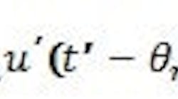
The model gain, Km, is the multiplier for the influence change that determines the new steady-state value for the PV. The FOPDT model pretends that once the delay duration, m, has passed, the PV follows a first-order exponential trajectory to the final steady-state value. The FOPDT time-constant, m, is an indicator of how fast the PV moves toward the new value. In contrast to some conventions, I used the subscript “m” for “model,” not the subscript “p” for “process,” to acknowledge that the model is not the process. I explicitly placed a squiggle hat over the model response variable, (t’), to indicate that it’s the model, not the process. And, I used the prime mark to indicate that the model influence, response and time are each a deviation from the initial steady conditions as well as the time for the step-and-hold influence. In figure 1, the change happens at a time of 155. Although t = 155, at that instant t’ = 0. Similarly, the initial process value is y = 37, but the deviation value is y’ = 0.
Although the concept for the model is a response to a step-and-hold influence from an initial steady state, and though this makes for convenient analytical solutions, it is a generic model, and not so restricted when solved with numerical methods. And, though the model can be equivalently stated in Laplace or z-transform notation, I won’t!
The classic textbook method to generate FOPDT models is the reaction curve technique, a pre-computer era method. It’s simple to understand and implement, and it can be derived from the analytical solution of the ODE, so it serves the current content of undergraduate engineering education appropriately. However, I believe reaction curve techniques don’t express best practices in the computer era.
However, a crude approximation FOPDT model is oftern all that’s needed. In such cases, a reaction curve technique can be a simple and fast method to get a good-enough model.
The reaction curve technique asks you to make a step-and-hold change in the process input, from an initial steady state, and hold the input until the response variable levels to an ending steady state. Unfortunately, noise and drifting alternate influences confound the response. And, a single step pushes the process away from a desired setpoint. Further, a push to one side of a nominal value will misrepresent nonlinear aspects. So, for effective reaction curve tests, we often use an up-down-down-up pattern in the influence step-and-hold values. This generates four reaction curves, and their average can temper the influence of noise and disturbances. Further, the pattern explores both sides of the original manipulated variable (MV) value, making compensating upsets and, ideally, returning the process to the original value.
These steps must be large enough to make a noticeable change in the response. If the change is small relative to normal noise and drifts, then the FOPDT model coefficients will have a large uncertainty.
Once the response curves are completed, the model coefficients are calculated from a few points on the response curve. There are multiple twists on the method.
However, this approach requires operator attention for an extended time to wait for four steady-state periods; may create process deviations that impact downstream quality; requires the human to interpret the signal to provide data for the mathematical analysis; only uses a small part of the data generated; and can be substantially confounded by uncontrolled disturbances.
In the computer era, by contrast, nonlinear least squares regression is simple to implement, and a skyline input function has advantages in operational duration, magnitude of upsets, and number of excitations over classical methods. A skyline pattern in the controller output could look like Figure 2.
[sidebar id =3]
The nonlinear regression method seeks to fit the model to all data points, not just the selected several points in a classic reaction curve fit. So, it better reject noise and disturbances.
The skyline and regression method does not require operator attention or judgment, which lessens the possibility for operator error or bias. And the skyline input has many ups and downs, which tempers the influence that environmental drifts have on confounding the CV response to the MV. The skyline and regression method does not extend the period of off-nominal production as each “+” or “-“ period is shorter, creating less objection by a quality manager. The skyline and regression method does not require an initial steady state, and the entire test period takes less time.
For a nonlinear process, gains, delays and time-constants change with MV and CV. The FOPDT model is linear, and may not provide a great match to the process over a wide operating range. Just because the optimizer converges on a best model, doesn’t mean that the model actually fits the data. So, after the regression, see if the fit is satisfactory for your model-use purposes.
[sidebar id =4]
Figure 3 reveals the data and best FOPDT model from the input sequence in Figure 2 for a pilot-scale process flow rate response to controller output. The model is the solid line, the data are the dots. It should be noted that early-time data is usually below the model, but late-time data is usually above. Perhaps some drifting influence was affecting the data.
In addition, note the kinks in the model at times a bit after 80 and 100. These are expected responses to small changes in the MV at those times, but these are not expressed in the data. Perhaps valve stiction prevented the valve from moving, even though the MV made changes. Finally, this data is not expected to be a linear response. Although the linear FOPDT model does not perfectly match the data, it’s also a very good representation of the process dynamics.
My Excel/VBA file for generating FOPDT models is posted at www.r3eda.com. It also offers a user guide to generate skyline data, use the software, and explain the nonlinear regression procedure. The VBA code is open. My entire academic career has been devoted to enabling students with best practices in engineering. I’m using the web site to extend beyond the classroom. I hope you find it useful.
[sidebar id =1]


