Monday morning you get a flood of emails saying that product quality is out the window, and you’re thinking of following it. There is a long line of batch operations between the raw materials and the final product. Lab samples show that product and byproduct endpoint concentrations of the batches have changed. The furthest upstream operation is a batch reactor. Something has changed in the fed batch reaction, but what? The process engineer says the reaction rate depends upon pressure, temperature, pH and concentrations. The data historian has no concentration measurements. A review of the trend charts shows that the pressure, temperature and pH are tightly controlled at their setpoints. You could probably tune the loops faster, but what is the point? The supplier spec sheets on the latest raw material shipments state everything is per the purchase orders. Is it time to retire to a tropical beach or pursue the management route so you can delegate the problem?
You are intrigued by the mystery so you start to look for clues. You reason that the control loops are doing a great job of transferring variability from the controlled variables (temperature, pressure and pH) to the manipulated variables (coolant, gas and liquid reactant, and reagent flows). The controller outputs appear much more interesting. The batch profiles of coolant, reactants and reagents flows show that their peaks are lower, offset and longer. The reagent profile also shows a long tail in the reagent flow. Why?
The “in-place” standardizations of the pH electrode indicate an offset between the pH at the start and end of the batch. A check with maintenance reveals a new electrode was installed at the start of the batch, and the reference electrode had not reached equilibrium with the process, which had a higher temperature and ionic strength than the buffers. The gradual change in the reference junction potential caused the long tail in the reagent flow. However, this tail is just part of the story. What caused the change in the width, location and maximum value of the peaks in the coolant, reactants and reagent flows?
Models are Knowledge
You can’t experiment with the plant because, even if it was not sold out, and the raw material and energy cost was justified, the review and paper work requirements would take too long. You turn to experimentation with a virtual plant. Within a few hours you find that flow profiles are symptomatic of changes in the reactant concentration. The model shows that some of the flows can be used as inferential measurements of reaction rate. The gaseous reactant feed rate under pressure control is proportional to reaction rate, since the pressure loop automatically adds reactant to make up for the reactant consumed. Additionally, you find coolant flow rate under temperature control is indicative of reaction rate because coolant makeup flow is compensating for the heat of reaction.
Making Do With What You Got
The makeup coolant temperature is tightly controlled at its setpoint. Everything points to a change in the raw materials. You can start to do extensive lab testing of each shipment, but that is too late for previous batches unless the problem persists. The ability to correlate lab results to future batches is not clear-cut since the lab analysis takes several hours and is done only during the day shift. The raw material shipments also enter the top of a storage tank, and the reactor is fed from the bottom. The degree of mixing from turbulence and equilibration is small, which creates a big transport delay from top to bottom.
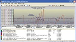
Figure 1. Effect of PID, feed-forward and sample time on glucose concentration control.
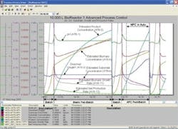
Since pressure, temperature and pH affect reaction rate, there is an opportunity for model-predictive control (MPC) to help maintain an inferential measurement of reaction rate at its maximum by the manipulation of these loop setpoints. A virtual plant shows that a prototype of the MPC performs well and leads to a reduction in cycle time.
Inferential measurements and soft sensors eventually need feedback correction, so you request lab tests be done periodically on a batch to provide an online adjustment. You reason that the number of batches you can wait in between special runs of lab analysis is a function of the trend in the corrections needed. Fortunately, in the case of reaction rates, the actual value is not as important as a directional relative indication of the changes in rate, which leads to the question: Is this the time for something much better for batch reactors?
Concentrating on Concentrations
Nearly all chemical and biological reaction rates depend upon the concentrations of the reactants, and quality depends upon the resulting product and byproduct concentrations. Yet you would be pressed to find off-line, let alone at-line or online concentration measurements of any components of reactants, products, byproducts or contaminants during any batch. The best kept secret of batch reactors is the concentration profiles.
In product development, the concentration profiles are measured in the lab with bench-top analyzers. The chemist or process development engineer knows the values of these profiles, but how can the need for this knowledge be realized and carried over to the commercial plant? A virtual plant can open minds and provide the justification for batch concentration profile analysis by prototyping advanced controls to make batch reaction rates more repeatable and faster. The virtual plant can also verify how fast you need concentration results from the analyzers to do closed loop control.
How Fast is Fast Enough?
The effect of analysis sample time comes down to the question of how much dead time can a sample add before feedback control noticeably deteriorates and causes instability. Intuitively you can understand that as the controller tuning slows down, the measurement speed required also slows down. Equation 1 documented at www.modelingandcontrol.com was developed to estimate when the sample dead time (ϴs) added to the original dead time (ϴo) makes the total loop dead time exceed the implied dead time from the controller tuning and causes the onset of degradation. The equation also estimates when the sample time gets so big it causes instability. The original equation was generalized to handle the pure integrating or “near-integrating” type of response of batch concentrations. Equation 1 shows that as you increase lambda (λ = closed loop time constant for self-regulating processes and the arrest time for integrating processes), the permissible amount of dead time (ϴs) from a sample increases for the standard PID algorithm.
ϴs ≤ Kx * (λ - ϴo ) (1)
Where:
ϴo = original dead time (sec)
ϴs = sample time (sec)
For self-regulating processes:
Kx = 0.5 for the start of degradation 2.0 for onset of instability
λ = closed loop time constant (sec)
For integrating processes:
Kx = 0.25 for the start of degradation 1.0 for onset of instability
λ = closed loop arrest time (sec)
To estimate the maximum allowable sample time that avoids the start of degradation and onset of instability, Kx is set equal to 0.5 and 2.0 for self-regulating and 0.25 and 1.0 for integrating processes, respectively in Equation 1. Lambda must be for the fastest response, which often depends upon its direction. For example, the glucose concentration response in a bioreactor is much faster for an increase in setpoint. The speed for a decrease in concentration depends upon the consumption rate. The attached plot from a virtual plant running 1000x real time shows that for glucose concentration control in a bioreactor, a sample time of about 11 hours causes oscillations with increasing amplitude (onset of instability) for a PID and an integrating response (Kx = 1.0) with a minimum closed-loop arrest time of 11 hours and a negligible original dead time. The figure shows that a PID algorithm enhancement for wireless control stabilizes the loop. The figure also illustrates how a feed-forward added to the PID output to pre-position the glucose flow for inoculation and increase the glucose flow with cell growth rate can considerably improve the glucose concentration control for both the standard and wireless PID, but feed-forward control could only delay, but not prevent, the eventual onset of instability for the standard PID.
The Max Slope is the Hope
Reactant and glucose concentration control also facilitates a more proficient design of experiments to identify kinetic parameters and an optimization of batch profiles by means of model-predictive control (MPC) since reaction, growth and formation rates depend upon these concentrations. For the identification of kinetic parameters, it is essential to use the slope instead of the actual product or cell concentration.
Figure 2. Reduction in batch cycle time by MPC production rate control
Table 1 lists candidates for controlled variables and manipulated variables for a bioreactor.
For many of the manipulated variables, the process action does not change between direct and reverse in the operating region. However, the pH and temperature optimum (peak in the plot of growth or formation rate versus pH or temperature) is narrow, so care must be taken to stay on one side of the peak to avoid a reversal in process action.
As the technology and availability of analyzers advances, you would think that exposing and controlling the secret profiles of batch reactors would be a top priority, since these reactors set the concentrations for downstream processes. In most cases, a slightly less-than-optimum profile would pay for a probe-type analyzer, and just one bad batch would pay for an at-line analyzer and sample system. So why maintain the status quo?
Top Ten Reasons to Keep Batch Reactor Concentration Profiles Secret
(10) Temperature and pressure is something you can feel
(9) Smart analyzers are too smart for their own good
(8) Everyone likes a good mystery
(7) Myths and war stories are interesting
(6) More meetings with catered lunches
(5) More creativity in performance reviews
(4) College texts on reaction kinetics are boring
(3) You can keep on trucking with PID control
(2) You can place bets on actual truck concentrations
(1) Purchasing is free to go with the lowest-cost supplier.
Greg McMillan is the coauthor of ControlTalk.

Leaders relevant to this article:


